from ssm4epi.models.regional_growth_factor import (
    key,
    n_iterations,
    N_mle,
    N_meis,
    N_posterior,
    percentiles_of_interest,
    make_aux,
    dates_full,
    cases_full,
    n_ij,
    n_tot,
    n_pop,
    account_for_nans,
    growth_factor_model,
)

from tqdm.notebook import tqdm
import pandas as pd

import jax.numpy as jnp
import jax
import jax.random as jrn

from isssm.importance_sampling import prediction
from isssm.laplace_approximation import laplace_approximation as LA
from isssm.modified_efficient_importance_sampling import (
    modified_efficient_importance_sampling as MEIS,
)

from pyprojroot.here import here

jax.config.update("jax_enable_x64", True)
from isssm.estimation import initial_theta
import pickle
import matplotlib.pyplot as plt
import pandas as pd
from datetime import date
min_date = date(2020, 10, 17)
max_date = date(2022, 1, 22)
np1 = 10
initial_dates = [
(d - pd.Timedelta(weeks=np1)).strftime("%Y-%m-%d")
for d in pd.date_range(start=min_date, end=max_date, freq="W-SAT", inclusive="both")
]
def initial_to_final_date(initial_date: date) -> date:
return initial_date + pd.Timedelta(weeks=np1)
final_dates = [
initial_to_final_date(pd.to_datetime(d)).strftime("%Y-%m-%d") for d in initial_dates
]
len(initial_dates)67def make_aux(date, cases_full, n_ij, n_tot, np1):
final_date = initial_to_final_date(pd.to_datetime(date))
df_weekly_cases = pd.read_csv(
here()
/ f"data/processed/RKI_county_{(final_date + pd.Timedelta(days=-5)).strftime('%Y-%m-%d')}.csv"
).pivot(index="date", columns="ags", values="cases")
cases_full = jnp.asarray(df_weekly_cases.to_numpy(), dtype=jnp.float64)
cases = cases_full[-(np1 + 1) :]
return cases, n_ij, n_totGLOBAL_KEY = jrn.PRNGKey(4534365463653)
def f_pred(x, s, y):
y_county = y[-1]
y_tot = jnp.minimum(y_county, n_pop).sum()[None]
growth_factors = s.reshape(-1)
return jnp.concatenate([y_tot, y_county, growth_factors])
def prediction_pipeline(initial_date):
(dates_index,) = jnp.where(dates_full == initial_date)[0]
dates = dates_full[dates_index : dates_index + np1]
aux = make_aux(initial_date, cases_full, n_ij, n_tot, np1)
y = aux[0][1:]
y_nan = y.at[-1].set(jnp.nan)
missing_inds = jnp.isnan(y_nan)
theta_manual = jnp.array(
# [5.950e00, -2.063e00, -5.355e00, -4.511e-01, -5.711e-01, 7.932e-01]
[0.0236392, -2.0838978, -5.31651543, -2.62109273, -0.3461143, 0.57673125]
)
_, y_miss = account_for_nans(
growth_factor_model(theta_manual, aux), y_nan, missing_inds
)
_model_miss = lambda theta, aux: account_for_nans(
growth_factor_model(theta, aux), y_nan, missing_inds
)[0]
theta0_result = initial_theta(
y_miss,
_model_miss,
theta_manual,
aux,
n_iter_la=n_iterations,
options={"maxiter": 10},
)
theta0 = theta0_result.x
fitted_model = _model_miss(theta0, aux)
proposal_la, _ = LA(y_miss, fitted_model, n_iterations)
key, subkey = jrn.split(GLOBAL_KEY)
preds = prediction(
f_pred,
y_miss,
proposal_la,
fitted_model,
1000,
subkey,
percentiles_of_interest,
growth_factor_model(theta0, aux),
)
result = (theta0, proposal_la, preds, dates, y)
with open(
here() / f"data/results/4_local_outbreak_model/results_{initial_date}.pickle",
"wb",
) as f:
pickle.dump(result, f)
df = pd.DataFrame(
{
"variable": [
"y_total",
*[f"y_total_{c}" for c in range(1, 401)],
*[f"log_rho_{c}_{t}" for t in range(1, 11) for c in range(1, 401)],
],
"c": [0, *range(1, 401), *[c for t in range(1, 11) for c in range(1, 401)]],
"t": [
10,
*jnp.repeat(10, 400),
*[t for t in range(1, 11) for c in range(1, 401)],
],
"mean": preds[0],
"sd": preds[1],
**{
f"{p * 100:.1f} %": preds[2][i, :]
for i, p in enumerate(percentiles_of_interest)
},
}
)
df["date"] = [dates[t - 1] for t in df["t"]]
df.to_csv(
here(f"data/results/4_local_outbreak_model/forecasts_{initial_date}.csv"),
index=False,
)def create_forecast_dataframe(initial_date):
with open(
here() / f"data/results/4_local_outbreak_model/results_{initial_date}.pickle",
"rb",
) as f:
result = pickle.load(f)
(theta0, proposal_la, _, dates, _) = result
(dates_index,) = jnp.where(dates_full == initial_date)[0]
dates = dates_full[dates_index : dates_index + np1]
aux = make_aux(initial_date, cases_full, n_ij, n_tot, np1)
y = aux[0][1:]
y_nan = y.at[-1].set(jnp.nan)
missing_inds = jnp.isnan(y_nan)
_, y_miss = account_for_nans(growth_factor_model(theta0, aux), y_nan, missing_inds)
_model_miss = lambda theta, aux: account_for_nans(
growth_factor_model(theta, aux), y_nan, missing_inds
)[0]
fitted_model = _model_miss(theta0, aux)
key, subkey = jrn.split(GLOBAL_KEY)
preds = prediction(
f_pred,
y_miss,
proposal_la,
fitted_model,
1000,
subkey,
percentiles_of_interest,
growth_factor_model(theta0, aux),
)
df = pd.DataFrame(
{
"variable": [
"y_total",
*[f"y_total_{c}" for c in range(1, 401)],
*[f"log_rho_{c}_{t}" for t in range(1, 11) for c in range(1, 401)],
],
"c": [0, *range(1, 401), *[c for t in range(1, 11) for c in range(1, 401)]],
"t": [
10,
*jnp.repeat(10, 400),
*[t for t in range(1, 11) for c in range(1, 401)],
],
"mean": preds[0],
"sd": preds[1],
**{
f"{p * 100:.1f} %": preds[2][i, :]
for i, p in enumerate(percentiles_of_interest)
},
}
)
df["date"] = [dates[t - 1] for t in df["t"]]
df.to_csv(
here(f"data/results/4_local_outbreak_model/forecasts_{initial_date}.csv"),
index=False,
)import jax.scipy as jsp
def make_theta_df(initial_date):
with open(
here() / f"data/results/4_local_outbreak_model/results_{initial_date}.pickle",
"rb",
) as f:
result = pickle.load(f)
(theta0, _, _, _, _) = result
logit_alpha, log_s2_r, log_s2_spat, logit_q, log_Cm1, log_r = theta0
return pd.Series(
{
"alpha": jsp.special.expit(logit_alpha),
"sigma_r": jnp.sqrt(jnp.exp(log_s2_r)),
"sigma spatial": jnp.sqrt(jnp.exp(log_s2_spat)),
"q": jsp.special.expit(logit_q),
"C": jnp.exp(log_Cm1) + 1,
"r": jnp.exp(log_r),
"date": initial_date,
}
)initial_dates[0]'2020-08-08'for initial_date in tqdm(initial_dates):
prediction_pipeline(initial_date)
create_forecast_dataframe(initial_date)df_params = pd.DataFrame([make_theta_df(date) for date in initial_dates])df_params| alpha | sigma_r | sigma spatial | q | C | r | date | |
|---|---|---|---|---|---|---|---|
| 0 | 0.5040491337848281 | 0.34439348042017437 | 0.07154196039249885 | 0.08052676729773568 | 1.5274437897836357 | 3.8703663450593546 | 2020-08-08 |
| 1 | 0.5052657454274464 | 0.34913894208280144 | 0.07079862141980918 | 0.07608048895422567 | 1.6637178130892964 | 3.996687630994572 | 2020-08-15 |
| 2 | 0.5005434268653365 | 0.33528463032010963 | 0.07400513431464514 | 0.06652954026176287 | 1.8489473680151751 | 4.609405663998974 | 2020-08-22 |
| 3 | 0.5046293866446885 | 0.3465898995999228 | 0.07144978090365359 | 0.060881711735945754 | 1.8523895369034156 | 5.3142547713105 | 2020-08-29 |
| 4 | 0.5058654690376462 | 0.3468133094609357 | 0.07169752434148507 | 0.056544238366418545 | 2.0369809103426526 | 5.950921053340124 | 2020-09-05 |
| ... | ... | ... | ... | ... | ... | ... | ... |
| 62 | 0.5522567924314707 | 0.3471588707436647 | 0.07466919009804708 | 0.021251505788375997 | 9.849538657594467 | 24.591565876595833 | 2021-10-16 |
| 63 | 0.5599998594568011 | 0.3473190516331426 | 0.07524648885516637 | 0.020455527118637882 | 10.220605039629321 | 27.24733431882475 | 2021-10-23 |
| 64 | 0.5655834786117435 | 0.3473476156463673 | 0.07629963970765477 | 0.02197164277281623 | 9.858752213079056 | 24.894234084807504 | 2021-10-30 |
| 65 | 0.5746749936151049 | 0.34812244531226416 | 0.0769235910937793 | 0.021452388220413118 | 8.99320216080605 | 21.734461384277903 | 2021-11-06 |
| 66 | 0.5705580393559064 | 0.34788586978226116 | 0.07569717711554107 | 0.023251338101012584 | 7.823244132814523 | 18.52382337645594 | 2021-11-13 |
67 rows × 7 columns
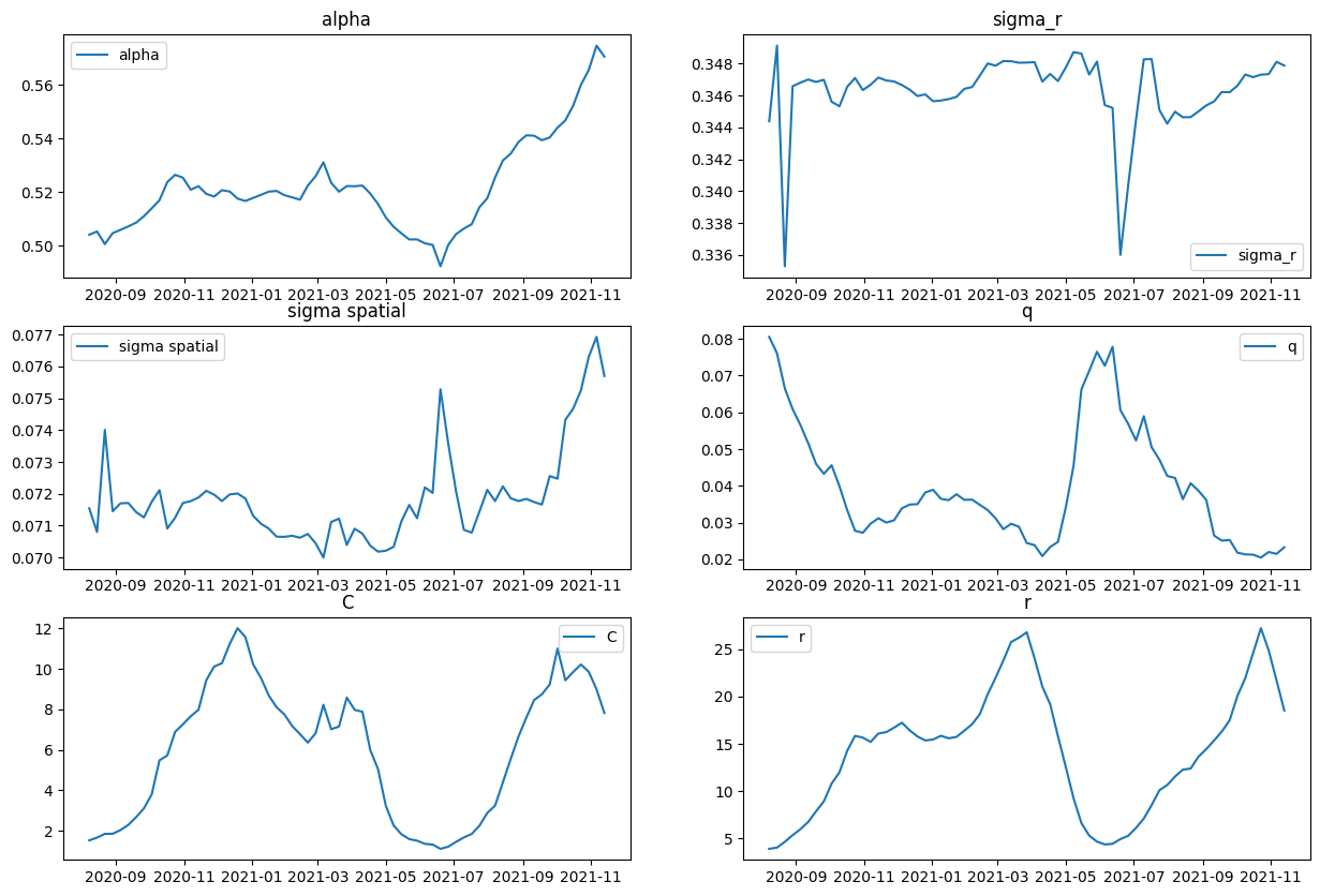
df_params["date"] = pd.to_datetime(df_params["date"])

plt.figure(figsize=(10, 6))
fig, axs = plt.subplots(3, 2, figsize=(15, 10))
for col, ax in zip(df_params.columns[:-1], axs.flatten()):
    ax.plot(df_params["date"], df_params[col], label=col)
    ax.set_title(col)
    ax.legend()
<Figure size 1000x600 with 0 Axes>